Estimating fitness using BiSSeCO

Introduction

This vignette will demonstrate how to to estimate within-host and between-host transmission fitness using the package musseco and the BiSSeCo (Binary-State Speciation and extinction Coalescent) model.

Basic requirements

This vignette assumes that you have the following packages already installed:

musseco: implements the likelihood function to estimate fitness.
ape: used for manipulation of phylogenetic trees.
TiPS: used to simulate a phylogenetic tree according to an epidemiological model.
ggplot2: used to visualize the results.

Load the necessary packages:

  library(musseco)
  library(TiPS)
  library(ape)
  library(ggplot2)

Simulated phylogenetic tree

To illustrate how we can use the R package musseco to estimate relative fitness, we will use a tree that was simulated with the R package TiPS.

This tree can be load as:

tr <- readRDS(system.file("extdata/tips_params_1_rep_2.rds", package = "musseco"))

Epidemiological model

This tree was simulate in a way that we know the true values of within-host and between-host replicative fitness.

The epidemiological model we used are described by the following equations, describing how the number of individuals carrying the ancestral ($Y_a$) and variant ($Y_v$) sequences changes with time.

$\dot{Y_a} = \beta Y_a (1 - \dfrac{N}{K}) + \mu_{va}Y_v - \mu_{av}Y_a - \gamma Y_a$

$\dot{Y_v} = \beta(1+s)Y_v (1 - \dfrac{N}{K}) - \mu_{va}Y_v + \mu_{av}Y_a - \gamma Y_v$

where the rate of new infections was defined as logistic growth controlled by the parameter $\beta$ for $Y_a(t)$ and $\beta(1+s)$, where $s$ is the selection coefficient, for $Y_v(t)$.

The carry capacity was defined by the parameter $K$ and was fixed at 10,000 individuals.

The rate $\mu_{av}$ defined how individuals carrying the ancestral state $Y_a(t)$ mutated to the $Y_v(t)$. The rate $\mu_{va}$ defined how individuals carrying the variant mutation reversed to the ancestral state, and this is also the molecular clock rate of evolution.

The rate $\gamma$ denoted the mortality rate.

In this vignette will not focus on how this tree was simulated, but the scripts to simulate the tree can be found here.

Table 1 shows the parameter values used to simulate the tree

Table 1: Parameter symbols and values
Parameter	Symbol	Values
Growth rate	$\beta$	0.216
Carrying capacity	$K$	10,000
Mortality rate	$\gamma$	1/10.2
Transition rate from $Y_v$ to $Y_a$	$\mu_{va}$	0.0016
Transition rate from $Y_a$ to $Y_v$	$\mu_{av}$	0.00176
Selection coefficient	$s$	-0.1
Between-host replicative fitness	$\omega$	0.9
Within-host replicative fitness	$\alpha$	1.1

Based on this parameter values, we know the true value of $\alpha$ and $\omega$.

Note that $\alpha = \mu_{av}/\mu_{va}$ and $\omega = 1 + s$.

Estimation of parameter values using fitbisseco

To estimate the within-host and between-host replicative fitness using the simulated phylogenetic tree, we will use the function fitbisseco from the musseco package.

Note that we need to define which tips of the phylogenetic tree carries the variant state.

isvariant <- grepl( tr$tip.label, pattern = 'V_' )
isvariant <- setNames(isvariant, tr$tip.label)

We also need to define the value of mu, which is the molecular clock rate of evolution. In our example, we used the rate for HIV-1 subtype C (Patiño-Galindo JÁ 2017) as we were modelling HIV-1 dynamics.

We also need to define the generation time (Tg). The generation time can be defined as $1/\gamma$.

Based on our Table 1, we know the values of mu and gamma.

# gamma value used in our epidemiological model
#Tg = 1/gamma
gamma <- 1/10.2
# mu (molecular clock) value used in our epidemiological model
mu <- 0.0016

Now we can run the fitbisseco function using the following command:

fb_au <- fitbisseco( tr,
                     isvariant,
                     Tg = 1/gamma,
                     mu = mu,
                     Net = NULL,
                     theta0 = log(c(2,.75,1/2)),
                     augment_likelihood = TRUE,
                     optim_parms = list(),
                     mlesky_parms = list(tau = NULL,
                                         tau_lower = 0.1,
                                         tau_upper = 1e7,
                                         ncpu = 1, 
                                         model = 1 ) )

Note the following options:

tr is the ape::phylo object, and this must be a time-scaled phylogeny.
isvariant vector of type boolean with lentgh equal to the number of tips in the phylogenetic tree. Each element is TRUE if the corresponding element in tr$tip.label is a variant type.
Tg is the generation time, i.e. the mean time elapsed between generations.
mu is the molecular clock rate of evolution;
Net (default NULL): but user can also provide a matrix with two columns giving the effective population size. If NULL, the effective population size will be computed with the mlesky R package. The first column should be time since some point in the past, and the second column should be an estimate of the effective population size. Time zero should correspond to the root of the tree.
theta0: Initial guess of (log) parameter values: alpha, omega, and Ne scale.

For details on the other parameters see ?musseco::fitbisseco.

But user can also provide additional parameter values to use with optim when fitting the model by maximum likelihood, mlskygrid function from the mlesky R package and the colik function from the phydynR package.

In addition, the fitbisseco function implements two types of likelihoods: the ‘coalescent’ and the ‘augmented’ likelihood. Both methods are based on the conditional density of a genealogy given epidemic and demographic parameters. The coalescent likelihood (by setting augment_likelihood = FALSE) relies solely on the phylogenetic tree to infer the fitness parameters. The augmented likelihood combines in a simple sum, the coalescent likelihood with a binomial likelihood of sampling variants or ancestral types under the assumption of random sampling and mutation-selection balance. The augmented likelihood is the default option in the fitbisseco function.

Obtaining the estimated parameter values

The fitbisseco function will take a few minutes to run. You can load the fit here

load(system.file("extdata/fit.rda", package = "musseco"))

fb_au
#> Binary state speciation and extinction coalescent fit
#> 
#>               2.5% 97.5%
#> alpha  0.910 0.570 1.453
#> omega  0.918 0.874 0.964
#> yscale 0.844 0.769 0.926
#> 
#> Likelihood: -5331.4195

We can now plot alpha and omega in respect to the true values listed in Table 1. The true values was those used to simulate the phylogenetic tree.

First we need to get the confidence interval as data.frame.

# threshold for approximate CIs 
MAXCOEFVAR <- 1.5

#variable names  
vnames <-  c('alpha', 'omega', 'yscale')
#the best values for the parameters found using optim
best_values <- coef(fb_au)[vnames]

# create a dataframe with the confidence interval
odf = as.data.frame(best_values)
odf$lower_bound <- exp( log(coef(fb_au)[vnames])-fb_au$err*1.96 )
odf$upper_bound <- exp( log(coef(fb_au)[vnames])+fb_au$err*1.96 )
odf$upper_bound[ fb_au$err > MAXCOEFVAR ] <- Inf
odf <- round( odf, 3 )

#add the true values to data.frame
odf["true_values"] <- c(1.1, 0.9, NA)
odf["Variable"] <- c("alpha", "omega", NA)
odf$Variable <- as.factor(odf$Variable)

#add a variable to data.frame to create a legend with ggplot2
odf["col1"] <- "Estimated values"
odf["col2"] <- "True values"
odf$col1 <- as.factor(odf$col1)
odf$col2 <- as.factor(odf$col2)

Plot we can plot the values for alpha and omega using ggplot.

  ggplot(odf[1:2,], aes(x = Variable)) +
  geom_point(aes(y = best_values, colour = col1), size = 3) +
  geom_errorbar(aes(ymax = upper_bound, ymin = lower_bound, 
                    width = 0.3, colour = col1)) +
  geom_point(aes(y = true_values, colour = col2) , size = 3) +
  facet_wrap( ~ Variable, scales = "free") +
  scale_color_manual(name = "",
                     values = c("Estimated values" = "#E69F00", 
                                "True values" =  "#009E73"), 
                     labels = c("Estimated values", "True values")) +
  theme_bw() +
  xlab("") +
  ylab("Confidence Interval") +
  theme(axis.text.x=element_blank(),
        axis.ticks.x=element_blank(),
        text = element_text(size = 20), 
        legend.position = "bottom")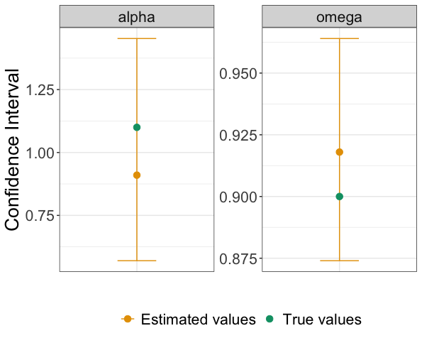

Bar plots showing the confidence interval for estimates of alpha and omega (in orange). True values for alpha and omega are depicted in green.

Figure 1: Bar plots showing the confidence interval for estimates of alpha and omega (in orange). True values for alpha and omega are depicted in green.

References

Patiño-Galindo JÁ, González-Candelas F. 2017. “The Substitution Rate of HIV-1 Subtypes: A Genomic Approach.” Virus Evolution 3 (2): vex029.

Fabricia F. Nascimento

2025-02-12