Estimating transmission rate using the SIR model

Introduction

This vignette will demonstrate how to use coalescent models as described in (Volz 2012) to estimate transmission rate parameters given a pathogen genealogy.

Basic requirements

This vignette assumes that you have the following packages already installed:

rjson: Converts R objects into JSON objects and vice-versa.
phydynR: implements the coalescent simulation and likelihood function for phylodynamics analysis
ggplot2: functions to plot the demographic process.

Load the necessary packages:

  library(phydynR)
  library(rjson)
  library(bbmle)
  library(ggplot2)

Suppose an epidemic occurs according to a density-dependent susceptible- infected-recovered (SIR) process, and a given infected individual generates a new infection at the rate $\beta SI$, where $S$ is the number susceptible and $\beta$ is the transmission rate. Furthermore, infected individuals will be removed from the population at per capita rate $\gamma$. At a single point in time, a random sample of $n = 75$ infected individuals is taken and the genealogy is reconstructed from the history of transmissions. We have simulated such a dataset using MASTER 1.10 (Vaughan and Drummond 2013), which can be loaded by

tree <- read.tree(system.file("extdata/sirModel0.nwk", package = "phydynR"))

And, the epidemic trajectory information can be loaded by

epidata <- rjson::fromJSON(file=system.file("extdata/sirModel0.json", package = "phydynR"))

The true parameter values are given in table 1. The file used to simulate the data with MASTER can be viewed by or directly openning the xml file.

file.show( system.file("extdata/sirModel0.xml", package = "phydynR"))

Table 1: Parameter symbols and values
Parameter	Symbol	Values
Duration infection	$1/\gamma$	1
Transmission rate	$\beta$	2.0002e-4
Population size	$S(0)$	9999
Initial num infected	$I(0)$	1
Time of sampling	$T$	12

We will fit a simple ordinary differential equation (ODE) model to the genealogy:

$\dot{S} = -\beta SI$

$\dot{I} = \beta SI -\gamma I$

Relevant parameters of the system are the transmission rate $\beta$, recovery rate $\gamma$, initial population size $S(0)$ and initial number infected $I(0)$. Not all parameters are identifiable from these data, so we will assume prior knowledge of $S(0)$ and $\gamma$ and focus on estimating $\beta$ and the nuisance parameter $I(0)$. Note that an imprecise estimate of $S(0)$ is also possible.

Create a list to store the true parameter values:


parms_truth <- list( beta = 0.00020002, 
                     gamma = 1, 
                     S0 = 9999, 
                     t0 = 0 )

Note that the true value of R0 is $\beta S(0)/\gamma = 2$.

And, create a tree with dated tips and internal nodes:


sampleTimes <- rep(12, 75)
names(sampleTimes) <- tree$tip.label

bdt <- DatedTree( phylo = tree, 
                  sampleTimes = sampleTimes)
bdt
#> 
#> Phylogenetic tree with 75 tips and 74 internal nodes.
#> 
#> Tip labels:
#>   24, 7, 36, 75, 52, 38, ...
#> 
#> Rooted; includes branch lengths.

Note that the vector of sample times must have names corresponding to the taxon labels in tree.

In order to fit this model, we need to express the equations in a canonical format:

births <- c( I = "beta * S * I" )
deaths <- c( I = "gamma * I" )
nonDemeDynamics <- c(S = "-beta * S * I")

The births vector gives the total rate that all infected generate new infections and deaths gives the rate that lineages are terminated. The nonDemeDynamics vector gives the equations for state variables that are not directly involved in the genealogy (e.g. because a pathogen never occupies a susceptible host by definition). Each element of the vectors is a string that will be parsed as R code and evaluated, so it is important to write it exactly as you would if you were solving the equations in R. Also note that the object parms is accessible to these equations, which is a list of parameters - this may include parameters to be estimated. Also note that we must give names to the vectors, and these names must correspond to the names of the demes.

We will use these initial conditions

# initial number of I and S
x0 <- c(I = 1, S = unname(parms_truth$S0))

# initial t0 (time of origin of the process)
t0 <- bdt$maxSampleTime - max(bdt$heights) - 1

The time of origin t0 is chosen somewhat arbitrarily, but should occur before the root of the tree.

The demographic model

After setting up all the components of the mathematical model, we can build the demographic process using the function build.demographic.process from the phydynR package. The dm output can be used as input to coalescent models for the calculation of the likelihood.

dm <- build.demographic.process(births = births,
                                nonDemeDynamics = nonDemeDynamics,
                                deaths = deaths,
                                parameterNames = names(parms_truth),
                                rcpp = TRUE,
                                sde = FALSE)
#> [1] "Thu Nov 28 15:08:11 2024 Compiling model..."
#> [1] "Thu Nov 28 15:08:16 2024 Model complete"

Now we can calculate the likelihood of the tree and assess how long it takes:

print(system.time(print(phydynR::colik(tree = bdt,
                                       theta = parms_truth,
                                       demographic.process.model = dm,
                                       x0 = x0,
                                       t0 = t0,
                                       res = 1000,
                                       integrationMethod = "rk4")
                        )))
#> [1] -378.142
#>    user  system elapsed 
#>   0.329   0.009   0.338

Note that changing the integrationMethod (choose “euler”), maxHeight (only fit to part of the tree) and res (set to a smaller value) options can dramatically speed up the calculation at the cost of some accuracy.

Fitting the model

We can fit the model using maximum likelihood with the bbmle or stats4 R packages.

obj_fun <- function(lnbeta, lnI0){
  
  beta <- exp(lnbeta)
  I0 <- exp(lnI0)
  parms <- parms_truth
  parms$beta <- beta
  x0 <- c(I = unname(I0), S = unname(parms$S0) )
  
  mll <- -phydynR::colik(tree = bdt,
                         theta = parms_truth,
                         demographic.process.model = dm,
                         x0 = x0,
                         t0 = t0,
                         res = 1000,
                         integrationMethod = "rk4")
  
  print(paste(mll, beta, I0))
  mll
}

Note that this uses log-transformation for variables that must be positive (like rates and population sizes). We can then fit the model by running

fit <- mle2(obj_fun,
            start = list(lnbeta = log(parms_truth$beta * 0.75), lnI0 = log(1)),
            method = "Nelder-Mead",
            optimizer = "optim",
            control = list(trace=6, reltol=1e-8))

Note that we are starting the optimizer far from the true parameter values. If fitting a model to real data, it is recommended to try many different starting conditions over a large range of values. The optimizer would take a few minutes to run, so instead we will load the results:

load( system.file("extdata/sirModel0-fit.RData", package="phydynR") )

AIC(fit)
#> [1] -145.7974
logLik(fit)
#> 'log Lik.' 74.89871 (df=2)
coef(fit)
#>     lnbeta       lnI0 
#> -8.4748155  0.1351695
exp(coef(fit))
#>       lnbeta         lnI0 
#> 0.0002086577 1.1447308446
exp(coef(fit)["lnbeta"]) - parms_truth$beta
#>       lnbeta 
#> 8.637689e-06

# how biased is the estimate?
exp(coef(fit)["lnbeta"]) - parms_truth$beta
#>       lnbeta 
#> 8.637689e-06

We can compare the fitted model to the true number of infected through time, which is shown in Figure 1.


beta <- exp(coef(fit)["lnbeta"])
I0 <- exp(coef(fit)["lnI0"])
parms <- parms_truth
parms$beta <- beta
x0 <- c(I = unname(I0), S = unname(parms$S0) )

o <- dm(parms,
        x0,
        t0,
        t1 = bdt$maxSampleTime,
        res = 1e3, 
        integrationMethod='rk4')
o <- o[[5]]

otruth <- dm(parms_truth,
             x0,
             t0, 
             t1 = bdt$maxSampleTime,
             res = 1e3, 
             integrationMethod='rk4')
otruth <- otruth[[5]]

rdata <- data.frame(time = epidata$t, I = epidata$I)

ggplot(rdata, aes(x = time, y = I)) +
  geom_point() +
  geom_line(data = o, aes(x = time, y = I), col='blue') +
  geom_line(data = otruth, aes(x = time, y = I), col='red') +
  theme_bw() +
  theme(element_text(size = 12)) +
  xlab("Time") +
  ylab("Number of infected")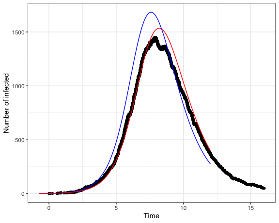

The actual (black) and estimated (red) number of infections through time. The blue line shows the SIR model prediction under the true parameter values.

Figure 1: The actual (black) and estimated (red) number of infections through time. The blue line shows the SIR model prediction under the true parameter values.

We can calculate a confidence interval for the transmission rate using likelihood profiles:

profbeta <- profile(fit, 
                    which = 1, 
                    alpha = 0.05,
                    std.err = 1, 
                    trace = TRUE,
                    tol.newmin = 1)

This takes a few minutes, so we will load the results:


load( system.file("extdata/sirModel0-profbeta.RData", package = "phydynR"))

We can see that the confidence interval covers the true value:


c( exp( confint( profbeta ) ), TrueVal = parms_truth$beta )
#>        2.5 %       97.5 %      TrueVal 
#> 0.0001901721 0.0002282366 0.0002000200

And, we can visualize the profile (Figure 2).

plot(profbeta)
abline( v = log( parms_truth$beta) , col = "red")

$Likelihood profile for the transmission rate $\beta$ with confidence levels. The true parameter value is indicated by the vertical red line.$

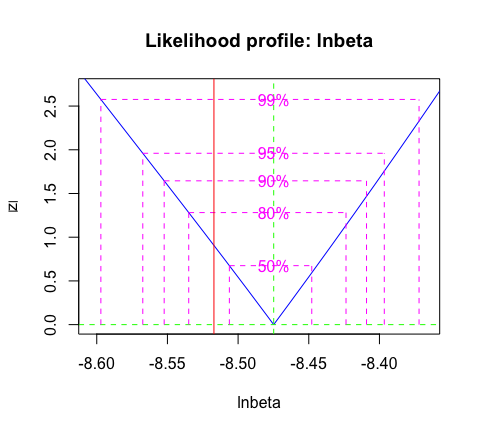
Figure 2: Likelihood profile for the transmission rate $\beta$ with confidence levels. The true parameter value is indicated by the vertical red line.

References

Vaughan, Timothy G., and Alexei J. Drummond. 2013. “A Stochastic Simulator of Birth–Death Master Equations with Application to Phylodynamics.” Molecular Biology and Evolution 30 (6): 1480–93. https://doi.org/10.1093/molbev/mst057.

Volz, Erik M. 2012. “Complex Population Dynamics and the Coalescent Under Neutrality.” Genetics 190 (1): 187–201. https://doi.org/10.1534/genetics.111.134627.

Erik Volz